Hello AHS: Run your first Analog Hamiltonian Simulation

AHS

Analog Hamiltonian Simulation (AHS) is a paradigm of quantum computing different from quantum circuits: instead of a sequence of gates, each acting only on a couple of qubits at a time, an AHS program is defined by the time- and space-dependent parameters of the Hamiltonian in question. The Hamiltonian of a system encodes its energy levels and the effects of external forces, which together govern the time evolution of its states. For an N-qubit systems, the Hamiltonian can be represented by a 2^NX2^N square matrix of complex numbers.

Quantum devices capable of performing AHS will tune their parameters (for example amplitude and detuning of a coherent driving field) to closely approximate the time evolution of the quantum system under the custom Hamiltonian. The AHS paradigm is suitable for simulating static and dynamic properties of quantum systems of many interacting particles. Purpose-built QPUs, such as the Aquila device from QuEra can simulate the time evolution of systems with sizes that are otherwise infeasible on classical hardware.

Interacting spin chain

For a canonical example of a system of many interacting particles, let us consider a ring of eight spins (each of which can be in “up” ∣↑⟩ and “down” ∣↓⟩ states). Albeit small, this model system already exhibits a handful of interesting phenomena of naturally occurring magnetic materials. In this example, we will show how to prepare a so-called anti-ferromagnetic order, where consecutive spins point in opposite directions.

Arrangement

We will use one neutral atom to stand for each spin, and the “up” and “down” spin states will be encoded in excited Rydberg state and ground state of the atoms, respectively. First, we create the 2-d arrangement. We can program the above ring of spins with the following code.

Prerequisites: You need to pip install the Braket SDK. (If you are using a Braket hosted notebook instance, this SDK comes pre-installed with the notebooks.) To reproduce the plots, you also need to separately install matplotlib with the shell command pip install matplotlib.

import numpy as np
import matplotlib.pyplot as plt  # required for plotting

from braket.ahs.atom_arrangement import AtomArrangement

a = 5.7e-6  # nearest-neighbor separation (in meters)

register = AtomArrangement()
register.add(np.array([0.5, 0.5 + 1/np.sqrt(2)]) * a)
register.add(np.array([0.5 + 1/np.sqrt(2), 0.5]) * a)
register.add(np.array([0.5 + 1/np.sqrt(2), - 0.5]) * a)
register.add(np.array([0.5, - 0.5 - 1/np.sqrt(2)]) * a)
register.add(np.array([-0.5, - 0.5 - 1/np.sqrt(2)]) * a)
register.add(np.array([-0.5 - 1/np.sqrt(2), - 0.5]) * a)
register.add(np.array([-0.5 - 1/np.sqrt(2), 0.5]) * a)
register.add(np.array([-0.5, 0.5 + 1/np.sqrt(2)]) * a)

which we can also plot with

fig, ax = plt.subplots(1, 1, figsize=(7,7))
xs, ys = [register.coordinate_list(dim) for dim in (0, 1)]
ax.plot(xs, ys, 'r.', ms=15)
for idx, (x, y) in enumerate(zip(xs, ys)):
    ax.text(x, y, f" {idx}", fontsize=12)
plt.show()  # this will show the plot below in an ipython or jupyter session

Interaction

To prepare the anti-ferromagnetic phase, we need to induce interactions between neighboring spins. We use the van der Waals interaction for this, which is natively implemented by neutral atom devices (such as the Aquila device from QuEra). Using the spin-representation, the Hamiltonian term for this interaction can be expressed as a sum over all spin pairs (j,k).

Here, nj​=∣↑_j​⟩⟨↑_j​∣ is an operator that takes the value of 1 only if spin j is in the “up” state, and 0 otherwise. The strength is V_j,k​=C₆​/(d_j,k​)⁶, where C₆​ is the fixed coefficient, and d_j,k​ is the Euclidean distance between spins j and k. The immediate effect of this interaction term is that any state where both spin j and spin k are “up” have elevated energy (by the amount V_j,k​). By carefully designing the rest of the AHS program, this interaction will prevent neighboring spins from both being in the “up” state, an effect commonly known as "Rydberg blockade."

Driving field

At the beginning of the AHS program, all spins (by default) start in their “down” state, they are in a so-called ferromagnetic phase. Keeping an eye on our goal to prepare the anti-ferromagnetic phase, we specify a time-dependent coherent driving field that smoothly transitions the spins from this state to a many-body state where the “up” states are preferred. The corresponding Hamiltonian can be written as

where Ω(t),ϕ(t),Δ(t) are the time-dependent, global amplitude (aka Rabi frequency), phase, and detuning of the driving field affecting all spins uniformly. Here S_−,k​=∣↓_k​⟩⟨↑_k​∣and S_+,k​​=(S_−,k​)^†=∣↑_k​⟩⟨↓_k​∣ are the lowering and raising operators of spin k, respectively, and n_k​=∣↑_k​⟩⟨↑_k​∣ is the same operator as before. The Ω part of the driving field coherently couples the “down” and the “up” states of all spins simultaneously, while the Δ part controls the energy reward for “up” states.

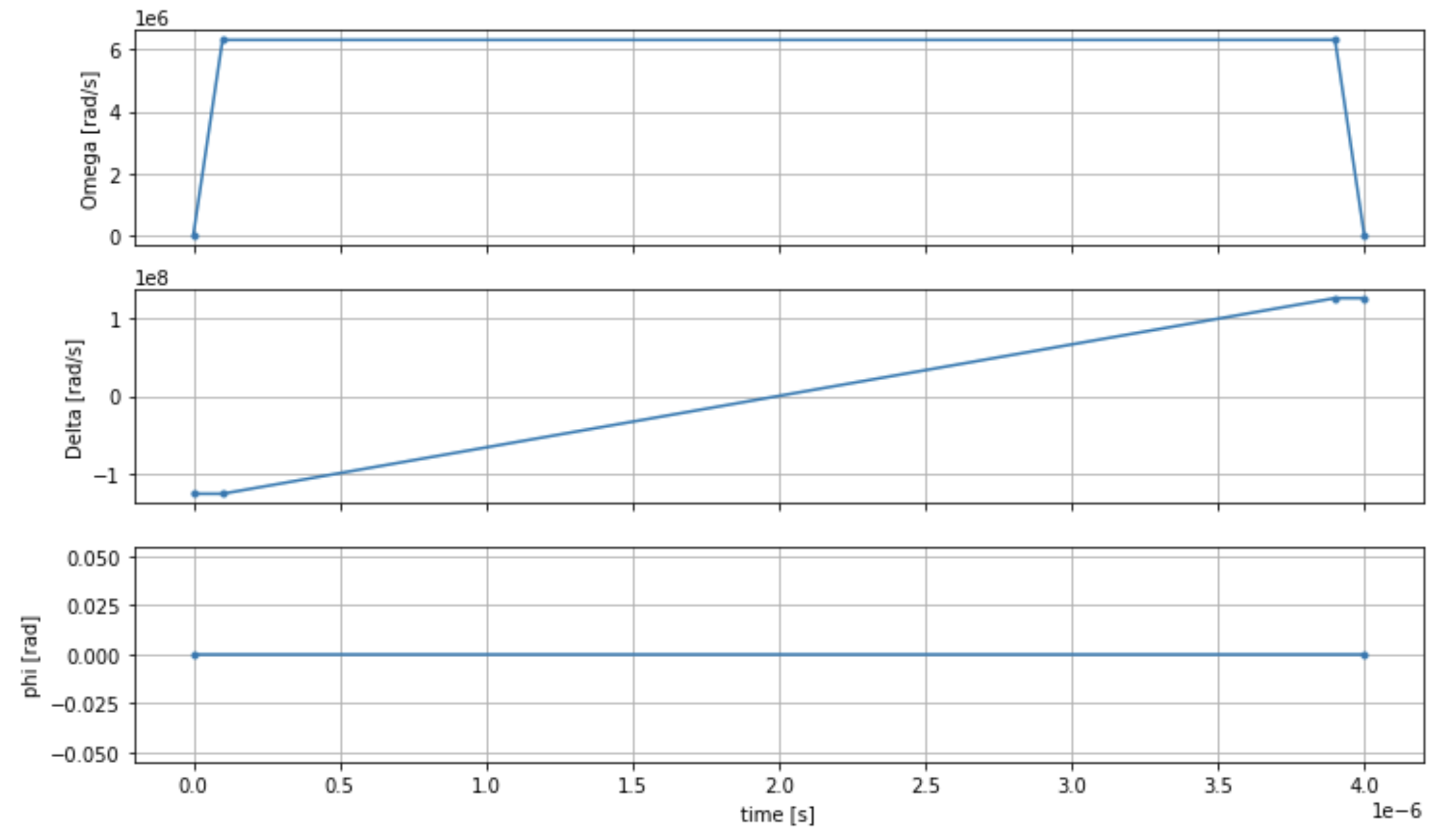
To program a smooth transition from the ferromagnetic phase to the anti-ferromagnetic phase, we specify the driving field with the following code.

from braket.timings.time_series import TimeSeries
from braket.ahs.driving_field import DrivingField

# smooth transition from "down" to "up" state
time_max = 4e-6  # seconds
time_ramp = 1e-7  # seconds
omega_max = 6300000.0  # rad / sec
delta_start = -5 * omega_max
delta_end = 5 * omega_max

omega = TimeSeries()
omega.put(0.0, 0.0)
omega.put(time_ramp, omega_max)
omega.put(time_max - time_ramp, omega_max)
omega.put(time_max, 0.0)

delta = TimeSeries()
delta.put(0.0, delta_start)
delta.put(time_ramp, delta_start)
delta.put(time_max - time_ramp, delta_end)
delta.put(time_max, delta_end)

phi = TimeSeries().put(0.0, 0.0).put(time_max, 0.0)

drive = DrivingField(
    amplitude=omega,
    phase=phi,
    detuning=delta
)

We can visualize the time series of the driving field with the following script.

fig, axes = plt.subplots(3, 1, figsize=(12, 7), sharex=True)

ax = axes[0]
time_series = drive.amplitude.time_series
ax.plot(time_series.times(), time_series.values(), '.-');
ax.grid()
ax.set_ylabel('Omega [rad/s]')

ax = axes[1]
time_series = drive.detuning.time_series
ax.plot(time_series.times(), time_series.values(), '.-');
ax.grid()
ax.set_ylabel('Delta [rad/s]')

ax = axes[2]
time_series = drive.phase.time_series
# Note: time series of phase is understood as a piecewise constant function
ax.step(time_series.times(), time_series.values(), '.-', where='post');
ax.set_ylabel('phi [rad]')
ax.grid()
ax.set_xlabel('time [s]')

plt.show()  # this will show the plot below in an ipython or jupyter session

AHS program

The register, the driving field, (and the implicit van der Waals interactions) make up the Analog Hamiltonian Simulation program ahs_program.

from braket.ahs.analog_hamiltonian_simulation import AnalogHamiltonianSimulation

ahs_program = AnalogHamiltonianSimulation(
    register=register,
    hamiltonian=drive
)

Running on local simulator

Since this example is small (less than 15 spins), before running it on an AHS-compatible QPU, we can run it on the local AHS simulator which comes with the Braket SDK. Since the local simulator is available for free with the Braket SDK, this is best practice to ensure that our code can correctly execute.

Here, we can set the number of shots to a high value (say, 1 million) because the local simulator tracks the time evolution of the quantum state and draws samples from the final state; hence, increasing the number of shots, while increasing the total runtime only marginally.

from braket.devices import LocalSimulator
device = LocalSimulator("braket_ahs")

result_simulator = device.run(
    ahs_program,
    shots=1_000_000
).result()  # takes about 5 seconds

Analyzing simulator results

We can aggregate the shot results with the following function that infers the state of each spin (which may be “d” for “down”, “u” for “up”, or “e” for empty site), and counts how many times each configuration occurred across the shots.

from collections import Counter

def get_counts(result):
    """Aggregate state counts from AHS shot results

    A count of strings (of length = # of spins) are returned, where
    each character denotes the state of a spin (site):
       e: empty site
       u: up state spin
       d: down state spin

    Args:
       result (braket.tasks.analog_hamiltonian_simulation_quantum_task_result.AnalogHamiltonianSimulationQuantumTaskResult)

    Returns
        dict: number of times each state configuration is measured

    """
    state_counts = Counter()
    states = ['e', 'u', 'd']
    for shot in result.measurements:
        pre = shot.pre_sequence
        post = shot.post_sequence
        state_idx = np.array(pre) * (1 + np.array(post))
        state = "".join(map(lambda s_idx: states[s_idx], state_idx))
        state_counts.update((state,))
    return dict(state_counts)

counts_simulator = get_counts(result_simulator)  # takes about 5 seconds
print(counts_simulator)

{'udududud': 330944, 'dudududu': 329576, 'dududdud': 38033, ...}

Here counts is a dictionary that counts the number of times each state configuration is observed across the shots. We can also visualize them with the following code.

from collections import Counter

def has_neighboring_up_states(state):
    if 'uu' in state:
        return True
    if state[0] == 'u' and state[-1] == 'u':
        return True
    return False

def number_of_up_states(state):
    return Counter(state)['u']

def plot_counts(counts):
    non_blockaded = []
    blockaded = []
    for state, count in counts.items():
        if not has_neighboring_up_states(state):
            collection = non_blockaded
        else:
            collection = blockaded
        collection.append((state, count, number_of_up_states(state)))

    blockaded.sort(key=lambda _: _[1], reverse=True)
    non_blockaded.sort(key=lambda _: _[1], reverse=True)

    for configurations, name in zip((non_blockaded,
                                    blockaded),
                                    ('no neighboring "up" states',
                                    'some neighboring "up" states')):
        plt.figure(figsize=(14, 3))
        plt.bar(range(len(configurations)), [item[1] for item in configurations])
        plt.xticks(range(len(configurations)))
        plt.gca().set_xticklabels([item[0] for item in configurations], rotation=90)
        plt.ylabel('shots')
        plt.grid(axis='y')
        plt.title(f'{name} configurations')
        plt.show()

plot_counts(counts_simulator)

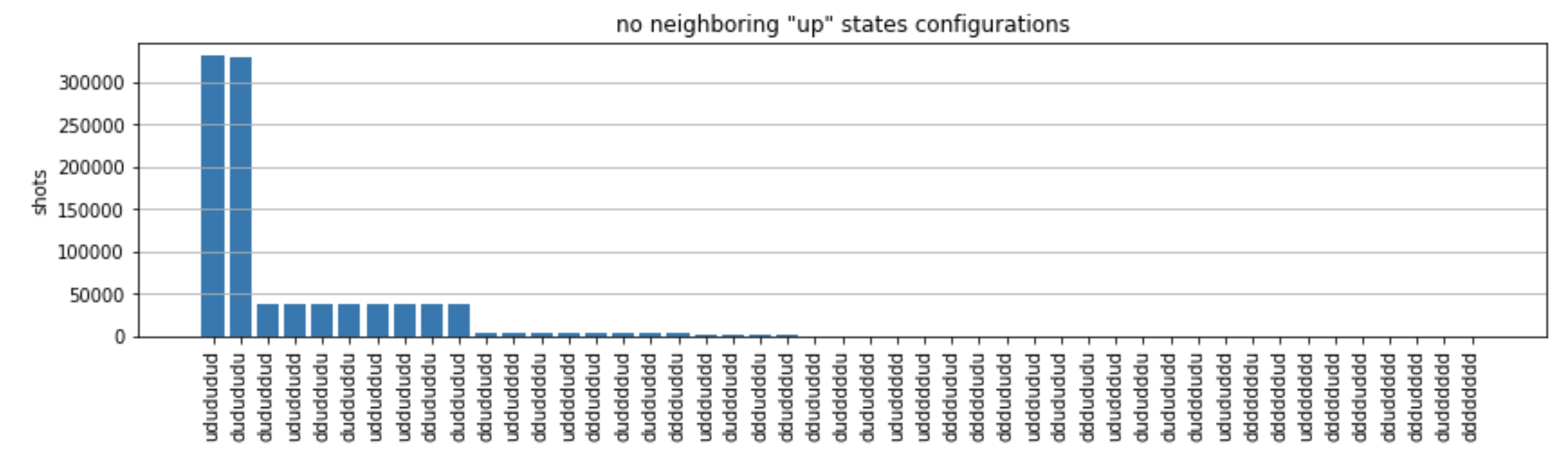
From the plots, we can read the following observations the verify that we successfully prepared the anti-ferromagnetic phase.

Running on QuEra’s Aquila QPU

Prerequisites: Apart from pip installing the Braket SDK, if you are new to Amazon Braket, please make sure that you have completed the necessary Get Started steps.

With all dependencies installed, we can connect to the Aquila QPU.

from braket.aws import AwsDevice

aquila_qpu = AwsDevice("arn:aws:braket:us-east-1::device/qpu/quera/Aquila")

To make our AHS program suitable for the QuEra machine, we need to round all values to comply with the levels of precision allowed by the Aquila QPU. (These requirements are governed by the device parameters with “Resolution” in their name. We can see them by executing aquila_qpu.properties.dict() in a notebook. For more details of capabilities and requirements of Aquila, see the Introduction to Aquila notebook.) We can do this by calling the discretize method.

discretized_ahs_program = ahs_program.discretize(aquila_qpu)

Now we can run the program (running only 100 shots for now) on the Aquila QPU.

task = aquila_qpu.run(discretized_ahs_program, shots=100)

metadata = task.metadata()
task_arn = metadata['quantumTaskArn']
task_status = metadata['status']

print(f"ARN: {task_arn}")
print(f"status: {task_status}")

task ARN: arn:aws:braket:us-east-1:123456789012:quantum-task/12345678-90ab-cdef-1234-567890abcdef
task status: CREATED

Due to the large variance of how long a quantum task may take to run (depending on availability windows and QPU utilization), it is a good idea to note down the quantum task ARN, so we can check its status at a later time with the following code snippet.

# Optionally, in a new python session

from braket.aws import AwsQuantumTask

SAVED_TASK_ARN = "arn:aws:braket:us-east-1:123456789012:quantum-task/12345678-90ab-cdef-1234-567890abcdef"

task = AwsQuantumTask(arn=SAVED_TASK_ARN)
metadata = task.metadata()
task_arn = metadata['quantumTaskArn']
task_status = metadata['status']

print(f"ARN: {task_arn}")
print(f"status: {task_status}")

*[Output]*
task ARN: arn:aws:braket:us-east-1:123456789012:quantum-task/12345678-90ab-cdef-1234-567890abcdef
task status: COMPLETED

Once the status is COMPLETED (which can also be checked from the quantum tasks page of the Amazon Braket console), we can query the results with:

result_aquila = task.result()

Analyzing QPU results

Using the same get_counts functions as before, we can compute the counts:

counts_aquila = get_counts(result_aquila)
print(counts_aquila)

*[Output]*
{'udududud': 24, 'dudududu': 17, 'dududdud': 3, ...}

and plot them with plot_counts:

plot_counts(counts_aquila)

Note that a small fraction of shots have empty sites (marked with “e”). This is due to a 1—2% per atom preparation imperfections of the Aquila QPU. Apart from this, the results match with the simulation within the expected statistical fluctuation due to small number of shots.

Next

Congratulations, you have now run your first AHS workload on Amazon Braket using the local AHS simulator and the Aquila QPU.

To learn more about Rydberg physics, Analog Hamiltonian Simulation and the Aquila device, refer to our example notebooks.