本文属于机器翻译版本。若本译文内容与英语原文存在差异，则一律以英文原文为准。

访问 Sentinel-2 栅格数据集合并创建地球观测作业以执行土地分割

这个基于 Python 的教程使用了 for SDK Python (Boto3) 和 Amazon Studio Classic 笔记本电脑。 SageMaker 要成功完成此演示，请确保您拥有使用 SageMaker 地理空间和 Studio Classic 所必需的 AWS Identity and Access Management (IAM) 权限。 SageMaker 地理空间要求您拥有可以访问 Studio Classic 的用户、群组或角色。您还必须在其信任策略sagemaker-geospatial.amazonaws.com中具有指定 SageMaker 地理空间服务主体的 SageMaker 执行角色。

要详细了解这些要求，请参阅SageMaker 地理空间IAM角色。

本教程向您展示如何使用 SageMaker 地理空间API来完成以下任务：

使用 list_raster_data_collections 查找可用的数据集合

SageMaker 地理空间支持多个栅格数据集合。要了解有关可用数据集合的更多信息，请参阅数据集合。

此演示使用从Sentinel-2云优化的地理卫星收集的TIFF卫星数据。这些卫星每五天对地球陆地表面进行一次全球覆盖。除了收集地球表面图像外，Sentinel-2 卫星还收集各种光谱带的数据。

要搜索感兴趣的区域 (AOI)，你需要与 Sentinel-2 卫星数据相关的区域。ARN要在中查找可用的数据集合及其关联ARNs数据 AWS 区域，请使用list_raster_data_collectionsAPI操作。

由于响应可以分页，因此必须使用 get_paginator 操作来返回所有相关数据：

import boto3
import sagemaker
import sagemaker_geospatial_map
import json 

## SageMaker Geospatial  is currently only avaialable in US-WEST-2  
session = boto3.Session(region_name='us-west-2')
execution_role = sagemaker.get_execution_role()

## Creates a SageMaker Geospatial client instance 
geospatial_client = session.client(service_name="sagemaker-geospatial")

# Creates a resusable Paginator for the list_raster_data_collections API operation 
paginator = geospatial_client.get_paginator("list_raster_data_collections")

# Create a PageIterator from the paginator class
page_iterator = paginator.paginate()

# Use the iterator to iterate throught the results of list_raster_data_collections
results = []
for page in page_iterator:
    results.append(page['RasterDataCollectionSummaries'])

print(results)

这是list_raster_data_collectionsAPI操作的示例JSON响应。该响应被截断，只包括此代码示例中使用的数据集合 (Sentinel-2)。有关特定栅格数据集合的更多详细信息，请使用 get_raster_data_collection：

{
    "Arn": "arn:aws:sagemaker-geospatial:us-west-2:378778860802:raster-data-collection/public/nmqj48dcu3g7ayw8",
    "Description": "Sentinel-2a and Sentinel-2b imagery, processed to Level 2A (Surface Reflectance) and converted to Cloud-Optimized GeoTIFFs",
    "DescriptionPageUrl": "https://registry.opendata.aws/sentinel-2-l2a-cogs",
    "Name": "Sentinel 2 L2A COGs",
    "SupportedFilters": [
        {
            "Maximum": 100,
            "Minimum": 0,
            "Name": "EoCloudCover",
            "Type": "number"
        },
        {
            "Maximum": 90,
            "Minimum": 0,
            "Name": "ViewOffNadir",
            "Type": "number"
        },
        {
            "Name": "Platform",
            "Type": "string"
        }
    ],
    "Tags": {},
    "Type": "PUBLIC"
}

运行前面的代码示例后，您将获得 Sentinel-2 栅格数据集合。ARN arn:aws:sagemaker-geospatial:us-west-2:378778860802:raster-data-collection/public/nmqj48dcu3g7ayw8在下一节中，您可以使用查询 Sentinel-2 数据集。search_raster_data_collection API

使用 search_raster_data_collection 搜索 Sentinel-2 栅格数据集合

在上一节中，您曾经list_raster_data_collections获取用于Sentinel-2数据收集的。ARN现在，您可以使用它ARN在给定的感兴趣区域 (AOI)、时间范围、属性和可用的 UV 波段上搜索数据集合。

要调用，search_raster_data_collectionAPI你必须向RasterDataCollectionQuery参数传Python入 dic 字典。此示例使用 AreaOfInterest、TimeRangeFilter、PropertyFilters 和 BandFilter。为方便起见，您可以使用变量 search_rdc_query 指定 Python 字典来保存搜索查询参数：

search_rdc_query = {
    "AreaOfInterest": {
        "AreaOfInterestGeometry": {
            "PolygonGeometry": {
                "Coordinates": [
                    [
                        # coordinates are input as longitute followed by latitude 
                        [-114.529, 36.142],
                        [-114.373, 36.142],
                        [-114.373, 36.411],
                        [-114.529, 36.411],
                        [-114.529, 36.142],
                    ]
                ]
            }
        }
    },
    "TimeRangeFilter": {
        "StartTime": "2022-01-01T00:00:00Z",
        "EndTime": "2022-07-10T23:59:59Z"
    },
    "PropertyFilters": {
        "Properties": [
            {
                "Property": {
                    "EoCloudCover": {
                        "LowerBound": 0,
                        "UpperBound": 1
                    }
                }
            }
        ],
        "LogicalOperator": "AND"
    },
    "BandFilter": [
        "visual"
    ]
}

在此示例中，您查询的 AreaOfInterest 包括犹他州的米德湖。此外，Sentinel-2 支持多种类型的图像波段。要测量水面的变化，您只需要 visual 波段即可。

创建查询参数后，您可以使用search_raster_data_collectionAPI来发出请求。

以下代码示例实现了search_raster_data_collectionAPI请求。这API不支持使用进行分页。get_paginator API为了确保已收集到完整的API响应，代码示例使用while循环来检查是否NextToken存在。然后，该代码示例用于.extend()将卫星图像URLs和其他响应元数据附加到。items_list

要了解更多信息search_raster_data_collection，请参阅SearchRasterDataCollection《亚马逊 SageMaker API参考》。

search_rdc_response = sm_geo_client.search_raster_data_collection(
    Arn='arn:aws:sagemaker-geospatial:us-west-2:378778860802:raster-data-collection/public/nmqj48dcu3g7ayw8',
    RasterDataCollectionQuery=search_rdc_query
)


## items_list is the response from the API request. 
items_list = []

## Use the python .get() method to check that the 'NextToken' exists, if null returns None breaking the while loop 
while search_rdc_response.get('NextToken'):
    items_list.extend(search_rdc_response['Items'])
    search_rdc_response = sm_geo_client.search_raster_data_collection(
        Arn='arn:aws:sagemaker-geospatial:us-west-2:378778860802:raster-data-collection/public/nmqj48dcu3g7ayw8',
        RasterDataCollectionQuery=search_rdc_query, NextToken=search_rdc_response['NextToken']
    )

## Print the number of observation return based on the query
print (len(items_list))

以下是您的查询的JSON回复。为清晰起见，该响应被截断。Assets 键值对中仅返回请求中指定的 "BandFilter": ["visual"]：

{
    'Assets': {
        'visual': {
            'Href': 'https://sentinel-cogs.s3.us-west-2.amazonaws.com/sentinel-s2-l2a-cogs/15/T/UH/2022/6/S2A_15TUH_20220623_0_L2A/TCI.tif'
        }
    },
    'DateTime': datetime.datetime(2022, 6, 23, 17, 22, 5, 926000, tzinfo = tzlocal()),
    'Geometry': {
        'Coordinates': [
            [
                [-114.529, 36.142],
                [-114.373, 36.142],
                [-114.373, 36.411],
                [-114.529, 36.411],
                [-114.529, 36.142],
            ]
        ],
        'Type': 'Polygon'
    },
    'Id': 'S2A_15TUH_20220623_0_L2A',
    'Properties': {
        'EoCloudCover': 0.046519,
        'Platform': 'sentinel-2a'
    }
}

现在您已经有了查询结果，在下一节中，您可以使用 matplotlib 对结果进行可视化。这是为了验证查询结果是否来自正确的地理区域。

使用 matplotlib 可视化 search_raster_data_collection

在开始地球观测作业 (EOJ) 之前，您可以使用可视化我们查询的结果matplotlib。以下代码示例从上一个代码示例中创建的 items_list 变量中获取第一项 items_list[0]["Assets"]["visual"]["Href"]，并使用 matplotlib 打印图像。

# Visualize an example image.
import os
from urllib import request
import tifffile
import matplotlib.pyplot as plt

image_dir = "./images/lake_mead"
os.makedirs(image_dir, exist_ok=True)

image_dir = "./images/lake_mead"
os.makedirs(image_dir, exist_ok=True)

image_url = items_list[0]["Assets"]["visual"]["Href"]
img_id = image_url.split("/")[-2]
path_to_image = image_dir + "/" + img_id + "_TCI.tif"
response = request.urlretrieve(image_url, path_to_image)
print("Downloaded image: " + img_id)

tci = tifffile.imread(path_to_image)
plt.figure(figsize=(6, 6))
plt.imshow(tci)
plt.show()

检查结果是否位于正确的地理区域后，可以在下一步中开始地球观测作业 (EOJ)。您可以使用称为土地分割的过程从卫星图像中识别水体。EOJ

开始对一系列卫星图像进行土地分割的地球观测工作 (EOJ)

SageMaker geospatial 提供了多个预训练模型，可用于处理来自栅格数据集合的地理空间数据。要了解有关可用的预训练模型和自定义操作的更多信息，请参阅操作类型。

要计算水面面积的变化，需要确定图像中哪些像素与水相对应。土地覆被分割是一种语义分割模型，由. start_earth_observation_job API 语义分割模型将标签与每张图像中的每个像素相关联。在结果中，每个像素都被分配了一个基于模型的类图的标签。以下是土地分割模型的类图：

{
    0: "No_data",
    1: "Saturated_or_defective",
    2: "Dark_area_pixels",
    3: "Cloud_shadows",
    4: "Vegetation",
    5: "Not_vegetated",
    6: "Water",
    7: "Unclassified",
    8: "Cloud_medium_probability",
    9: "Cloud_high_probability",
    10: "Thin_cirrus",
    11: "Snow_ice"
}

要开始地球观测作业，请使用start_earth_observation_jobAPI。当您提交请求时，必须指定以下内容：

InputConfig 是一个 Python 字典。使用下面的变量 eoj_input_config 来保存搜索查询参数。在start_earth_observation_jobAPI发出请求时使用此变量。w.

# Perform land cover segmentation on images returned from the Sentinel-2 dataset.
eoj_input_config = {
    "RasterDataCollectionQuery": {
        "RasterDataCollectionArn": "arn:aws:sagemaker-geospatial:us-west-2:378778860802:raster-data-collection/public/nmqj48dcu3g7ayw8",
        "AreaOfInterest": {
            "AreaOfInterestGeometry": {
                "PolygonGeometry": {
                    "Coordinates":[
                        [
                            [-114.529, 36.142],
                            [-114.373, 36.142],
                            [-114.373, 36.411],
                            [-114.529, 36.411],
                            [-114.529, 36.142],
                        ]
                    ]
                }
            }
        },
        "TimeRangeFilter": {
            "StartTime": "2021-01-01T00:00:00Z",
            "EndTime": "2022-07-10T23:59:59Z",
        },
        "PropertyFilters": {
            "Properties": [{"Property": {"EoCloudCover": {"LowerBound": 0, "UpperBound": 1}}}],
            "LogicalOperator": "AND",
        },
    }
}

JobConfig是一个字Python典，用于指定要对数据执行的EOJ操作：

eoj_config = {"LandCoverSegmentationConfig": {}}

现在指定了字典元素后，您可以使用以下代码示例提交start_earth_observation_jobAPI请求：

# Gets the execution role arn associated with current notebook instance 
execution_role_arn = sagemaker.get_execution_role()

# Starts an earth observation job
response = sm_geo_client.start_earth_observation_job(
    Name="lake-mead-landcover",
    InputConfig=eoj_input_config,
    JobConfig=eoj_config,
    ExecutionRoleArn=execution_role_arn,
)
            
print(response)

启动地球观测任务会返回ARN以及其他元数据。

要获取所有正在进行和当前的地球观测工作的清单，请使用 list_earth_observation_jobsAPI. 要监控单个地球观测任务的状态，请使用 get_earth_observation_jobAPI. 要提出此请求，请在提交EOJ请求后使用ARN创建的。要了解更多信息，请参阅 GetEarthObservationJobAmazon SageMaker API 参考文档。

要查找与您ARNs关联的，EOJs请使用list_earth_observation_jobsAPI操作。要了解更多信息，请参阅 ListEarthObservationJobsAmazon SageMaker API 参考文档。

# List all jobs in the account
sg_client.list_earth_observation_jobs()["EarthObservationJobSummaries"]

以下是JSON响应示例：

{
    'Arn': 'arn:aws:sagemaker-geospatial:us-west-2:111122223333:earth-observation-job/futg3vuq935t',
    'CreationTime': datetime.datetime(2023, 10, 19, 4, 33, 54, 21481, tzinfo = tzlocal()),
    'DurationInSeconds': 3493,
    'Name': 'lake-mead-landcover',
    'OperationType': 'LAND_COVER_SEGMENTATION',
    'Status': 'COMPLETED',
    'Tags': {}
}, {
    'Arn': 'arn:aws:sagemaker-geospatial:us-west-2:111122223333:earth-observation-job/wu8j9x42zw3d',
    'CreationTime': datetime.datetime(2023, 10, 20, 0, 3, 27, 270920, tzinfo = tzlocal()),
    'DurationInSeconds': 1,
    'Name': 'mt-shasta-landcover',
    'OperationType': 'LAND_COVER_SEGMENTATION',
    'Status': 'INITIALIZING',
    'Tags': {}
}

EOJ作业状态更改为后COMPLETED，继续下一节以计算湖泊Mead's 表面积的变化。

计算米德湖表面积的变化

要计算米德湖表面积的变化，请先使用export_earth_observation_job以下方法将结果导出EOJ到 Amazon S3：

sagemaker_session = sagemaker.Session()
s3_bucket_name = sagemaker_session.default_bucket()  # Replace with your own bucket if needed
s3_bucket = session.resource("s3").Bucket(s3_bucket_name)
prefix = "export-lake-mead-eoj"  # Replace with the S3 prefix desired
export_bucket_and_key = f"s3://{s3_bucket_name}/{prefix}/"

eoj_output_config = {"S3Data": {"S3Uri": export_bucket_and_key}}
export_response = sm_geo_client.export_earth_observation_job(
    Arn="arn:aws:sagemaker-geospatial:us-west-2:111122223333:earth-observation-job/7xgwzijebynp",
    ExecutionRoleArn=execution_role_arn,
    OutputConfig=eoj_output_config,
    ExportSourceImages=False,
)

要查看导出作业的状态，请使用 get_earth_observation_job：

export_job_details = sm_geo_client.get_earth_observation_job(Arn=export_response["Arn"])

要计算米德湖水位的变化，请将土地覆盖掩码下载到本地 n SageMaker otebook 实例，然后从我们之前的查询中下载源图像。在土地分割模型的类图中，水体的类指数为 6。

要从 Sentinel-2 图像中提取水遮罩，请按照以下步骤操作。首先，计算图像中标记为水（类指数为 6）的像素数。其次，将计数乘以每个像素所覆盖的面积。波段的空间分辨率可能有所不同。对于土地覆被分割模型，所有波段均向下采样至等于 60 米的空间分辨率。

import os
from glob import glob
import cv2
import numpy as np
import tifffile
import matplotlib.pyplot as plt
from urllib.parse import urlparse
from botocore import UNSIGNED
from botocore.config import Config

# Download land cover masks
mask_dir = "./masks/lake_mead"
os.makedirs(mask_dir, exist_ok=True)
image_paths = []
for s3_object in s3_bucket.objects.filter(Prefix=prefix).all():
    path, filename = os.path.split(s3_object.key)
    if "output" in path:
        mask_name = mask_dir + "/" + filename
        s3_bucket.download_file(s3_object.key, mask_name)
        print("Downloaded mask: " + mask_name)

# Download source images for visualization
for tci_url in tci_urls:
    url_parts = urlparse(tci_url)
    img_id = url_parts.path.split("/")[-2]
    tci_download_path = image_dir + "/" + img_id + "_TCI.tif"
    cogs_bucket = session.resource(
        "s3", config=Config(signature_version=UNSIGNED, region_name="us-west-2")
    ).Bucket(url_parts.hostname.split(".")[0])
    cogs_bucket.download_file(url_parts.path[1:], tci_download_path)
    print("Downloaded image: " + img_id)

print("Downloads complete.")

image_files = glob("images/lake_mead/*.tif")
mask_files = glob("masks/lake_mead/*.tif")
image_files.sort(key=lambda x: x.split("SQA_")[1])
mask_files.sort(key=lambda x: x.split("SQA_")[1])
overlay_dir = "./masks/lake_mead_overlay"
os.makedirs(overlay_dir, exist_ok=True)
lake_areas = []
mask_dates = []

for image_file, mask_file in zip(image_files, mask_files):
    image_id = image_file.split("/")[-1].split("_TCI")[0]
    mask_id = mask_file.split("/")[-1].split(".tif")[0]
    mask_date = mask_id.split("_")[2]
    mask_dates.append(mask_date)
    assert image_id == mask_id
    image = tifffile.imread(image_file)
    image_ds = cv2.resize(image, (1830, 1830), interpolation=cv2.INTER_LINEAR)
    mask = tifffile.imread(mask_file)
    water_mask = np.isin(mask, [6]).astype(np.uint8)  # water has a class index 6
    lake_mask = water_mask[1000:, :1100]
    lake_area = lake_mask.sum() * 60 * 60 / (1000 * 1000)  # calculate the surface area
    lake_areas.append(lake_area)
    contour, _ = cv2.findContours(water_mask, cv2.RETR_TREE, cv2.CHAIN_APPROX_SIMPLE)
    combined = cv2.drawContours(image_ds, contour, -1, (255, 0, 0), 4)
    lake_crop = combined[1000:, :1100]
    cv2.putText(lake_crop, f"{mask_date}", (10,50), cv2.FONT_HERSHEY_SIMPLEX, 1.5, (0, 0, 0), 3, cv2.LINE_AA)
    cv2.putText(lake_crop, f"{lake_area} [sq km]", (10,100), cv2.FONT_HERSHEY_SIMPLEX, 1.5, (0, 0, 0), 3, cv2.LINE_AA)
    overlay_file = overlay_dir + '/' + mask_date + '.png'
    cv2.imwrite(overlay_file, cv2.cvtColor(lake_crop, cv2.COLOR_RGB2BGR))

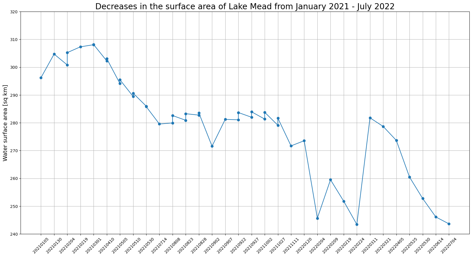
# Plot water surface area vs. time.
plt.figure(figsize=(20,10))
plt.title('Lake Mead surface area for the 2021.02 - 2022.07 period.', fontsize=20)
plt.xticks(rotation=45)
plt.ylabel('Water surface area [sq km]', fontsize=14)
plt.plot(mask_dates, lake_areas, marker='o')
plt.grid('on')
plt.ylim(240, 320)
for i, v in enumerate(lake_areas):
    plt.text(i, v+2, "%d" %v, ha='center')
plt.show()

使用 matplotlib，您可以通过图表直观显示结果。从图中可以看出，2021 年 1 月至 2022 年 7 月，米德湖面积有所减少。